Metal Surface Defect Detection

This project was carried out as part of the TechLabs “Digital Shaper Program” in Aachen (Summer Term 2022)

Introduction

Quality inspection and control in the steel-manufacturing industry have been critical issues for assuring product quality and increasing productivity. As a steel defect is deemed to be one of the main causes of the increase in production cost, monitoring the quality of steel products is inevitable during the manufacturing process [1]. The defects can be attributed to various factors, e.g., operational conditions and facilities [2]. For an immediate response and control of the flaws, detecting steel defects should be preceded to analyse the failure causes. To this end, a sophisticated diagnostic model is required to detect the failures properly and to enhance the capability of quality control [3].

The traditional human inspection system has several disadvantages such as less autonomy and time-consuming procedure [4]. In particular, a vision-based diagnostics system for detecting steel surface defects has received considerable attention. An image-based system, on the other hand, is developed to enable more elaborate, rapid, and automatic inspection than the existing methods [5].

It is widely known that the surface defect accounts for more than 90% of entire defects in steel products, e.g., plate and strip [6]. Defects on the steel surface, e.g., scratches, patches, and inclusions exert a maleficent influence on material properties, i.e., fatigue strength and corrosion resistance, as well as the appearance [7]. Likewise, the development of a visual inspection system for identifying steel surface defects should be conducted to secure the reliability of the process and the product.

Over recent years, a variety of research based on machine learning and deep learning techniques have been conducted to establish a defect diagnostics model of the steel surface with machine vision, showing feasible performance for an automatic inspection system.

In this work, two improved computational model named ==ResNet-50 convolutional neural network & VGG16 convolutional neural network== is proposed for surface defect images of hot rolled strip [8]. Furthermore, Generative adversarial networks (GANs) are algorithmic architectures that use two neural networks, pitting one against the other (thus the “adversarial”) to generate new, synthetic instances of data that can pass for real data. A new GAN-based classification method for detecting surface defects of strip steel is proposed. The GANs are used to generate more data sets to bloat the training images to make the model more robust [9].

Dataset

The NEU surface defect dataset was readily available on the Kaggle Open-source Dataset website in which, six kinds of typical surface defects of the hot-rolled steel strip are collected, i.e., rolled-in scale (RS), patches (Pa), crazing (Cr), pitted surface (PS), inclusion (In) and scratches (Sc). The database includes 1,800 grayscale images: 300 samples each of six different kinds of typical surface defects.

Surface defect dataset

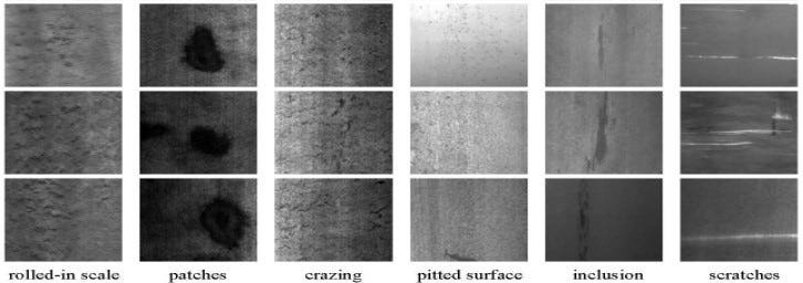
Figure shows the sample images of six kinds of typical surface defects, the original resolution of each image is 200×200 pixels. The defects are varied according to structure, size, and shape, for instance, the scratches (the last column) may be horizontal scratch, vertical scratch, slanting scratch, etc. On the other hand, some defects have similar aspects, e.g., rolled-in scale, crazing, and pitted surface.

The given data is categorised randomly into three sub-folders namely Training, Testing, and Validation respectively. The training dataset consists of 276 images of each defect and 12 images are taken for testing and validation dataset.

Methodology

Although several studies have been conducted to enhance the defect detection performance in the steel surface, there are still challenging issues for practical use, which motivates this study.

Firstly, the local binary patterns (LBP) method with SVM has been employed due to the merits of low computational complexity, meticulous descriptive quality, and illumination variation robustness [10]. Secondly, tuning the hyper-parameters and building the optimised architectural structure is carried out to maximise the classification performance for detecting the steel surface defects [11]. Moreover, the transfer learning approach is also discussed with two improved convolutional neural network computational models named ==ResNet-50 & VGG16==. In addition to that, a GAN-based classification method for detecting surface defects of strip steel is carried out to generate more data.

2.1. Support Vector Machines (SVM)

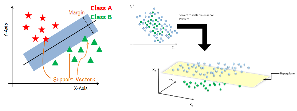
SVM is a supervised learning method used for solving multi-class classification and regression problems. Recently it has gained an exceedingly good reputation as a machine learning algorithm for classification in medicine and engineering fields. It can easily handle multiple continuous and categorical variables. SVM generates an optimal hyperplane iteratively, to minimise misclassification error. The core idea of SVM is to find a maximum marginal hyperplane that best divides the dataset into classes.

SVM maps data to high-dimensional feature space for better categorisation, when linearly not separable. As the dimensions of the feature plane are increased for better categorisation, the separators are no more lines but hyperplanes. Such manipulations of input data done by mathematical functions are called Kernel functions [12].

Support vector machine visualisation

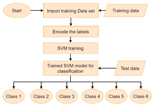
2.1.1 SVM on Training Data

Firstly, SVM is directly employed in the training dataset. The Image matrix is flattened and provided to SVM for training. The working of the algorithm can be deduced from figure.

SVM training process

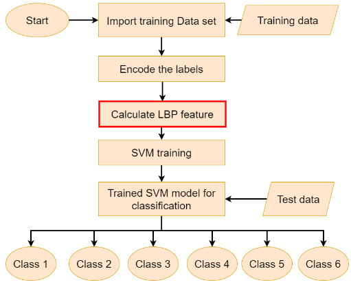
2.1.2 SVM with Feature extraction (Local binary pattern)

There are two important issues to be addressed: 1 — Effective defect features must be explored, extracted, and optimised. Defect features characterise surface defects and determine the complexity of the classification system. 2 — Classifier design, which determines the performance of the entire vision system in classifying defects. Support Vector Machine did address this issue.

For the first issue, we choose Local Binary Pattern (LBP). LBP is a Texture pattern descriptor introduced by Ojala et. al[13] to describe the local texture patterns of an image. LBP is computed as a binary encoding of differences in pixel intensities with the local neighbourhood. The reference process is illustrated in the following figure.

LBPrn = 1, Irn ≥ Io = 0, Irn < Io Io = intensity of a pixel, Irrn = intensity of neighbourhood “n” refers to the position of neighbour 1 ≤ n ≤ 8, with n = 1 to the right of the centre pixel, and increasing in an anticlockwise direction. “r” denotes the radius of neighbour's considered. r = 1 here.

Feature extraction from 3x3 neighbourhood

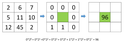
A similar computation is performed for every pixel in the image and a histogram of these values is created to form the LBP feature. Since a 3 x 3 neighbourhood has 28 = 256 possible patterns, our LBP 2D array thus has a minimum value of 0 and a maximum value of 255, allowing us to construct a 256-bin histogram that tabulates the frequency of each LBP pattern that occurred. We then sum bin sizes of the histogram and normalize it, this is our final feature vector[14]. SVM with LBP implementation is deduced by following diagram.

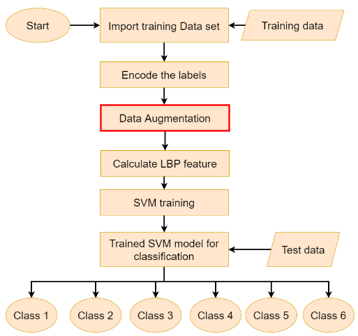
2.1.3 SVM with Feature extraction (Local binary pattern) and Image Augmentation.

The SVM with LBP Feature Extraction method produced improved results compared to standard deployment. To further improve the model image augmentation techniques such as rotation are employed on the dataset and then augmented images fed to SVM with LBP Feature Extractor. The reference process flow chart depicts the process of SVM with LBP Feature Extractor for the augmented image dataset.

2.2 Convolutional Neural Networks (Hyper Parameter Tuning)

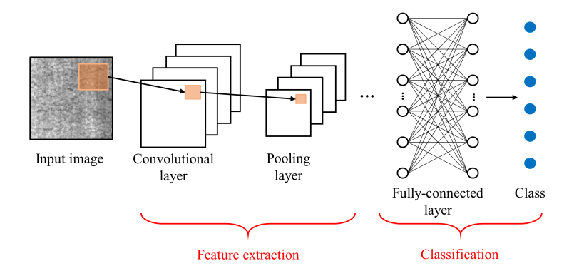
SVM indeed provide a low computational cost solution to the problem, but convolutional neural networks are traditionally popular for image classification task. A convolutional neural network (CNN) is a type of deep neural network which uses successive operations across a variety of layers, which is specified to deal with a two-dimensional image. CNN, firstly introduced in [15], is known to be a successful neural network algorithm for image processing and recognition. The CNN architecture is typically made up of two main stages, feature extraction, and classification. Extracted feature representations are fed into the latter part of the architecture, where the model depicts a probability of belonging to a certain class. Likewise, the weights and biases of the model are optimized by training the neural network via the back-propagation algorithm.

Typical Architecture of CNN’s

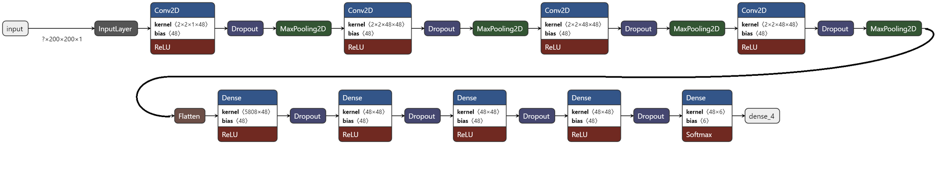
Keras Tuner is a hyper-parameter optimisation framework that solves the pain points of performing a hyper-parameter search to find the best hyper-parameter values. Bayesian optimisation, one of the types of hyper-parameter tuning, is a probabilistic model that maps the hyper-parameters to a probability score on the objective function by keeping track of its past evaluation results and using it to build the probability model. The model is trained several times for different activation functions, input units, and dropouts until the best model is selected. The ==best model architecture== is as follows-

Best model architecture

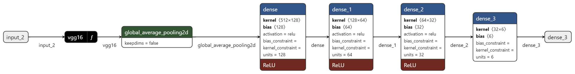
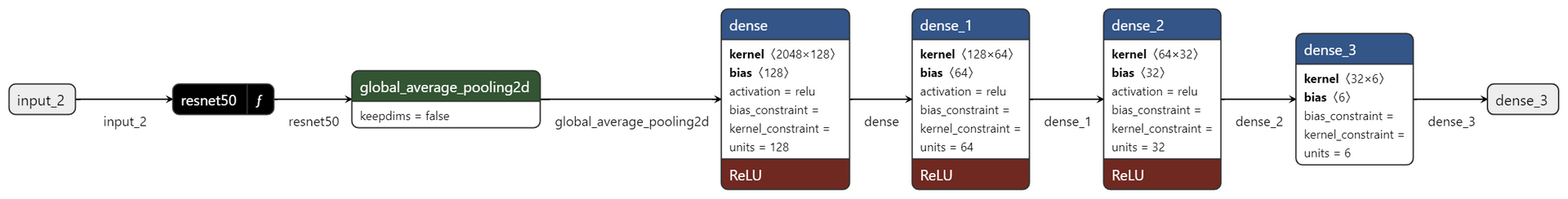
2.3 Convolutional Neural Networks (Transfer Learning)

Transfer learning is generally used to save time and resources from having to train multiple machine learning models from scratch to complete similar tasks as in the previous case. Transfer learning can be understood as applying knowledge from a previous task to a new task. Based on the theory of transfer learning, we can achieve small-scale defect image data sets classification by decomposing and changing the large-scale CNN networks pre-trained on ImageNet [16].

In general, existing strip surface defect classification networks tend to use off-the-shelf deep learning network structures and their various variants, including AlexNet, VGGNet, GoogleNet, ResNet, DenseNet, SENet, ShuffleNet, MobileNet, etc. Compared with traditional algorithms such as machine learning, deep learning algorithms have higher accuracy; however, deep learning often requires a larger amount of data.

2.3.1 Data Augmentation

Data Augmentation is a way to ensure that the model doesn’t treat the object as different in case it is subjected to small variations like rotation, variations in lighting conditions, etc. By applying data augmentation, the diversity increases, the learning process is boosted and it makes the model robust. The following data augmentation techniques were used: — RandomContrast — RandomFlip(mode=“horizontal_and_vertical”), — RandomZoom — RandomRotation — RandomTranslation

By using these techniques the model is further employed for training.

2.3.2 Model Training

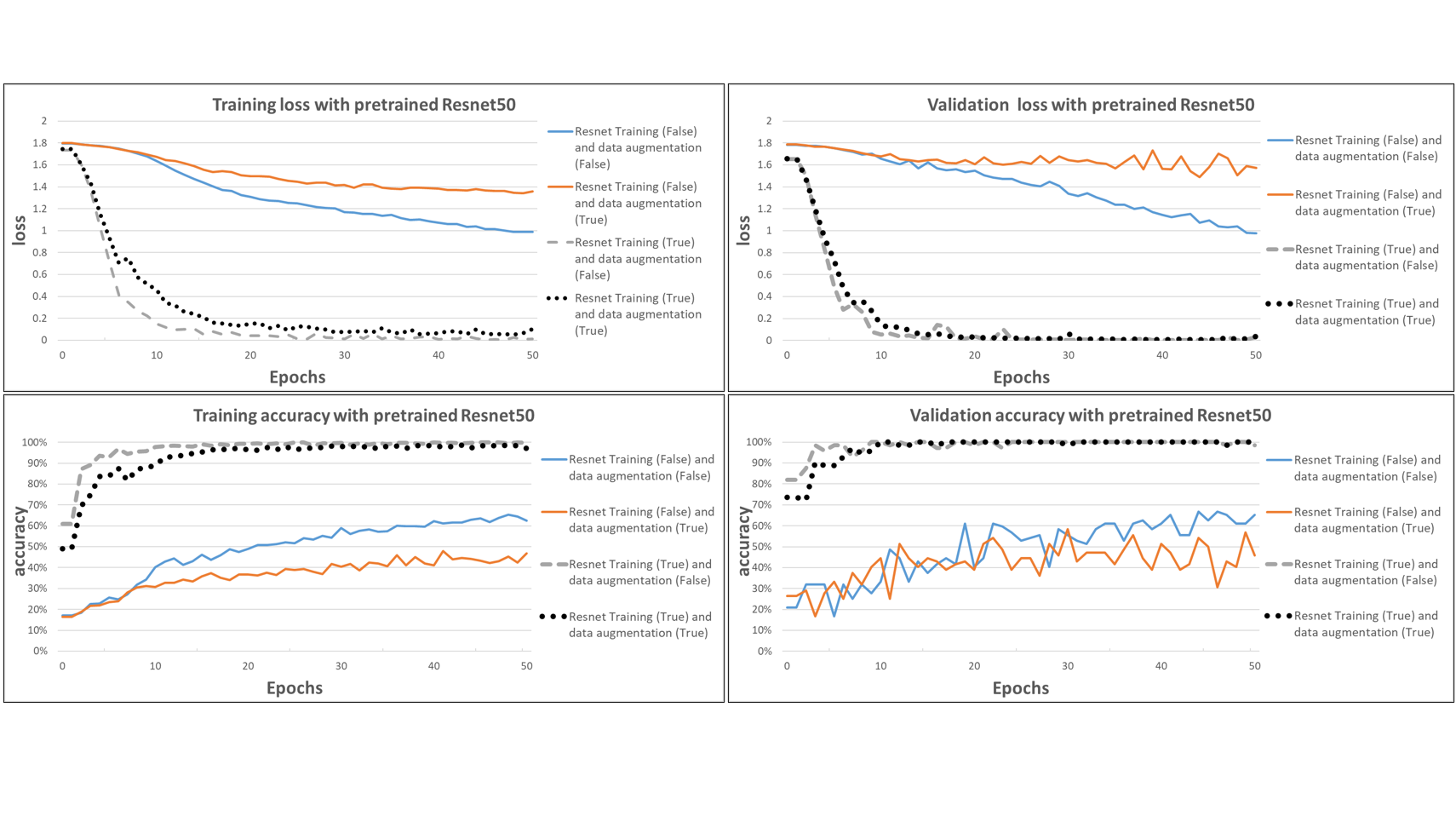
The models were subjected to 4 cases respectively: 1. VGG16/Resnet50 during training were not trained but the rest of the layers were trained with no data augmentation. 2. VGG16/Resnet50 during training were not trained but the rest of the layers were trained with data augmentation. 3. All layers of the model including VGG16/Resnet50 were trained with no data augmentation. 4. All layers of the model including VGG16/Resnet50 were trained with data augmentation.

The models were iterated for 50 epochs with the Adam optimizer. The learning rate of 0.0001 was set for the modified Resnet50 model and 0.0005 for the modified VGG16 model using the idea of a learning rate finder from fast.ai. The model was run for 1 epoch with varied learning rates learning rate. The point where the slope changes maximum before the loss rises again is selected as the learning rate for faster learning. The best model architecture is as follows-

VGG16_training_false_aug_false (2).h5.png

Resnet50 without training and without augmentation

2.4 Generative Adversarial Networks (GANs)

The lack of high-quality steel strip defect datasets makes the effectiveness of deep learning in steel strip defect classification somewhat limited. Thus, A new GAN-based classification method for detecting surface defects of strip steel is proposed. GANs work by training a generator network that outputs synthetic data. The generative model captures the data distribution of the training data to generate the synthetic data. This synthetic data is then run through the discriminator network to get a gradient. The discriminative model here estimates the probability that the synthetic data is from the training sample or the generator [17]. The gradient indicates how much the synthetic data needs to change for it to look/represent data that is more realistic than representing data or an image that is synthetically generated.

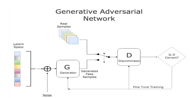
2.4.1 Conditional GANs (cGANs)

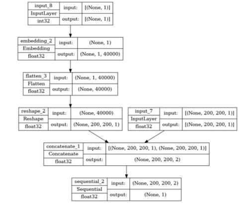
The inspiration for the application of a conditional GANs network was solely due to the lack of diversity of data in the available data set. This resulted in the application of conditional GANs over conventional GANs as it would have been advantageous for the project to generate synthetic data relevant for each class. Hence, targeted image generation was important which gave reason for the application of conditional GANs. The Conditional-GANs model slightly modifies the conventional GAN architecture by adding a label parameter to the input of the generator on which the generator can condition on [18]. There is also an additional label parameter for the discriminator to distinguish the real data better.

Various tutorials help developers implement the conditional GANs using python, one of which was used in this project [19]. In this project, we merely have 300 images of size (200, 200) for each defect of hot-rolled steel. After defining the number of classes as six, the generator model function definition is created to accommodate the new size image. The model itself is a CNN network with 3 convolution layers, with a couple of LeakyReLU activations. The general architecture can be described as the generation of an image for a particular label based on a combination of latent vectors and its label (conditional GANs).

GAN 1

The discriminator architecture is responsible for classifying if the image is real or generated based on a probabilistic scale. This again is a combination of CNN consisting of convolution layers, LeakyReLU activation, and the last layer being a sigmoid activation for classification after which training function with different iterations and batch sizes are defined.

GAN 2

3. Result and Discussion

In this section, the results of the employed methods are shown and discussed. Each result is compared with one another based on performance metrics such as the confusion matrix and classification report. Using these performance metrics we can depict the best model suitable for the classification of surface defects of hot-rolled steel. On the other hand, GANs are used to generate fake images, and then these fake images are employed in the discriminator model.

3.1 Support Vector Machines (SVM)

After training on each method proposed, the model is evaluated and deployed based on two performance metrics i.e. Classification Matrix and Classification Report

3.1.1 SVM on Training Data

The Classification Report and Confusion matrix are as follows:

SVM Reports and Confusion Matrices

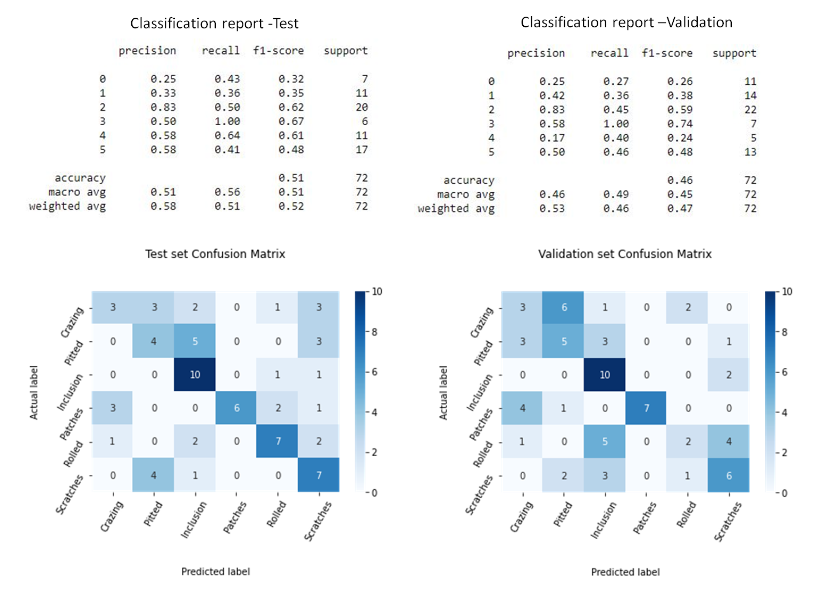
Based on performance metrics we can deduce that when SVM is directly employed on the raw data available, the accuracy and classification are not up to the mark (51% for test data and 46% for validation data). Hence there is a need to find a suitable feature extraction method.

3.1.2 SVM with Feature extraction (Local binary pattern)

The Classification Report and Confusion matrix are as follows:

SVM with Feature Extraction Reports and Confusion Matrices

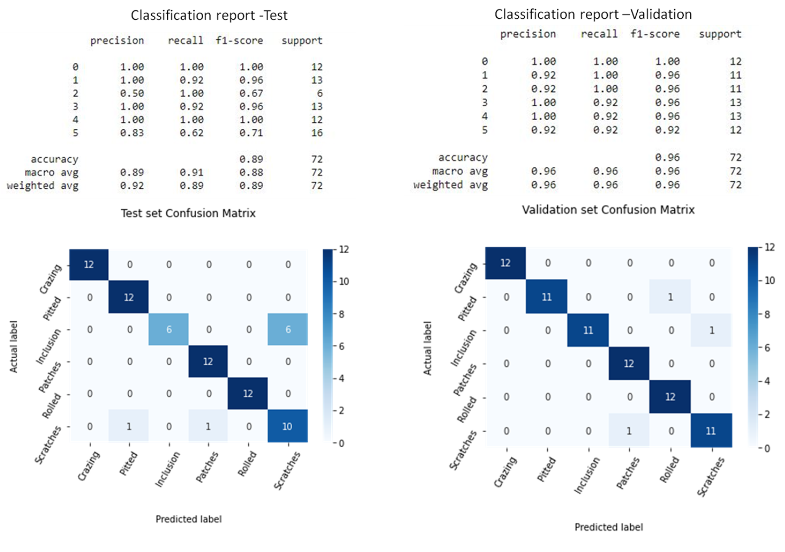
The performance metric shows considerable improvement in results with LBP as a feature extractor with raw data. The test and validation results are much better compared to previous results (89% for test data and 96% for validation data). To further improve the model, data augmentation is employed.

3.1.3 SVM with Feature extraction (Local binary pattern) and Image Augmentation

The Classification Report and Confusion matrix are as follows:

Reports and Confusion Matrices

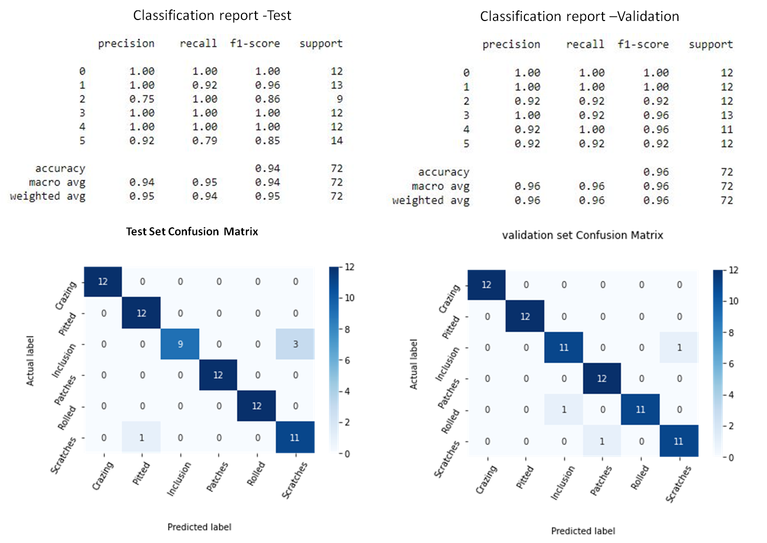
Based on the results obtained, the accuracy and classification for the test dataset are significantly improved (94% for test data) but for validation data, no changes are observed. To establish a suitable model for classification, deep learning methods are used for classification.

3.2 Convolutional Neural Networks

The Convolutional Neural Networks are trained by using two methods viz., hyperparameter tuning and transfer learning. CNN provides holistic results compared to SVM which are discussed in the following section.

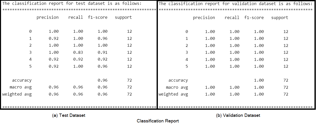
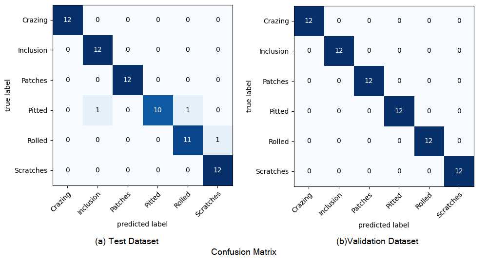
3.2.1 CNN — Hyper Parameter Tuning

The prediction accuracy of the model is illustrated in the classification report for the training and validation dataset, it can be seen that the best model achieves the best classification performance with the accuracy of 95.83% with a loss of 0.099, and only 3 images were misclassified for test images and no misclassification for validation dataset. The confusion matrix is shown to show the classification effect of each kind of defect more carefully. It can be seen that the model can achieve 100% of classification accuracy for all six defects for the validation dataset.

Though the model showed the best results possible, the model was trained several times. Therefore, to save time and resources from having to train multiple machine learning models from scratch transfer learning methods are outlooked.

3.2.2 Transfer Learning

Transfer learning is where we take architectures like VGG16 and ResNet50 which are the result of extensive hyperparameter tuning and apply that knowledge to a new task instead of starting from scratch.

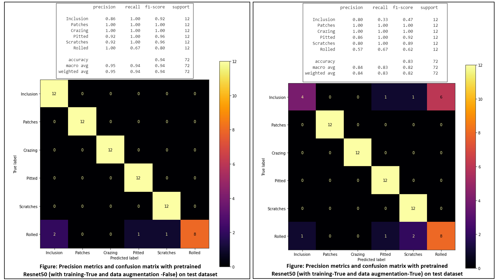
• ResNet50

The model was explored for the following 4 cases:

• When Resnet50 was not trained but the rest of the layers were trained with no data augmentation. (Training- False and data augmentation-False)
• When Resnet50 was not trained but the rest of the layers were trained with data augmentation. (Training- False and data augmentation-True)
• When all layers including Resnet50 were trained with no data augmentation (Training- True and data augmentation-False)
• When all layers including Resnet50 were trained with data augmentation (Training- True and data augmentation-True)

From the training and accuracy curves, the best performance was observed when all the layers of the model were trained with and without augmentation. They are robust and the losses and accuracy of the training and validation are set to converge.

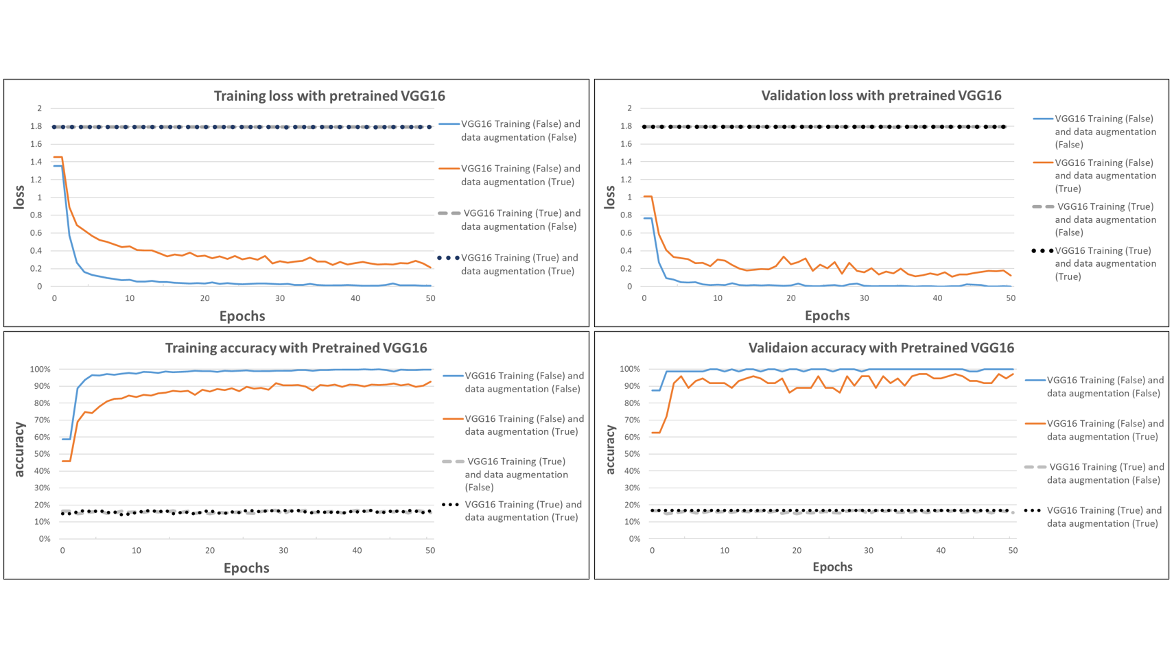
• VGG16

The model was explored for the following 4 cases: — When VGG16 was not trained but the rest of the layers were trained with no data augmentation (Training- False and data augmentation-False) — When VGG16 was not trained but the rest of the layers were trained with data augmentation (Training- False and data augmentation-True) — When all layers including VGG16 were trained with no data augmentation (Training- True and data augmentation-False) — When all layers including VGG16were trained with data augmentation (TrainingTrue and data augmentation-True)

From the training and accuracy curves, the best performance was observed when the layers of the model except VGG16 were trained with and without augmentation. They are robust and the losses and accuracy of the training and validation are set to converge. The model got stuck at local minima during training when VGG16 was included in the training.

3.3 Generative Adversarial Networks (GANs)

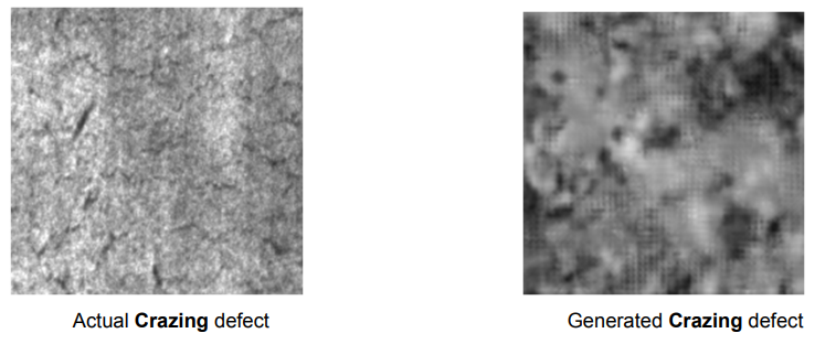
Unfortunately, the results of the generated images did not serve the required purpose of bloating the training image set. Different methods were attempted:

1. Just feed one class training data and see if the generated image were close to the real ones
2. Change the optimizer to see if the results get better
3. Use of data augmentation methods while training the GAN model

None of the above attempts succeeded in generating relevant images for the defects. Below is an example of different images generated for the defect Crazing.

Sample of crazing defect

4. Conclusion

SVM alone had poor prediction accuracy when directly employed on the training dataset. But, the prediction accuracy of SVM increased drastically in couple with feature extractors LBP. Moreover, the accuracy is further increased by 5% when data augmentation is performed on the dataset resulting in 94% accuracy. For further improvement of prediction accuracy, deep learning methods like CNN with Hyperparameter Tuning and Transfer learning are employed.

The hyper-tuned CNN model performed 95.83% accurately on the test dataset with the augmented training dataset. On the other hand, it has performed exceptionally for the validation dataset. To compensate computational power the transfer learning approach is selected for the same results as the low-cost model.

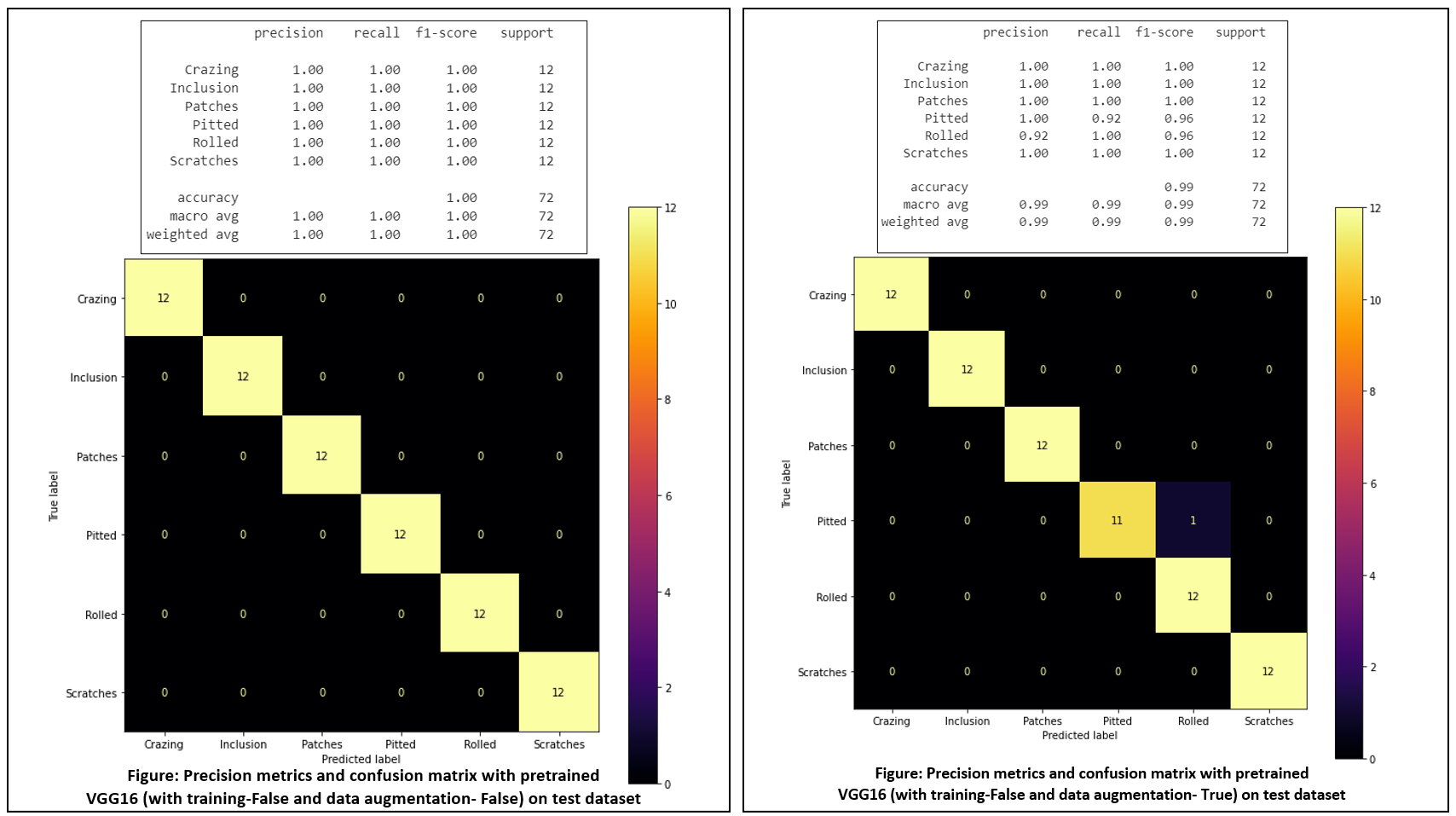
Two transfer learning models were employed on data viz. VGG16 and ResNet50 for different conditions. VGG16 when not trained with the rest of the layers with no data augmentation turned out to be the best model achieving 100% accuracy on the test dataset.

The usage of cGANs, although understandable, did not result in the best of results. This can be primarily attributed to a few reasons:

1. GANs in themselves require a lot of data. Considering just 1800 images for 6 classes resulted in an under performing model
2. The GAN model could have been constructed from scratch drawing inspiration from the latest models that have worked well with less data
3. Other generative models could have been explored

To conclude, machine learning and deep learning approaches were discussed in this project for the classification of surface defects of hot-rolled steel. Support Vector Machines performed better with augmented images and LBP feature extractors with lesser time than both CNN models. On the other hand, both CNN models outperformed SVM in terms of accuracy and loss rate. The model with tuned parameters was computationally expensive hence transfer learning approach is selected, which showed the same result. The prediction time for each model is almost similar. The GANs, on the other hand, did not perform as per expectation and could be improved with other generative models.

The goal of this project was to obtain the best classification model for the given task. VGG16 (with 100% accuracy) is proven to be most suitable model for the given task. The team’s coordinated effort helped in achieving this goal.

References

1. Song, G.W.; Tama, B.A.; Park, J.; Hwang, J.Y.; Bang, J.; Park, S.J.; Lee, S. Temperature Control Optimization in a Steel-Making Continuous Casting Process Using Multimodal Deep Learning Approach. Steel Res. Int. 2019, 90, 1900321.
2. Luo, Q.; He, Y. A cost-effective and automatic surface defect inspection system for hot-rolled flat steel. Robot. Comput.-Integr. Manuf. 2016, 38, 16–30.
3. Ghorai, S.; Mukherjee, A.; Gangadaran, M.; Dutta, P.K. Automatic defect detection on hot-rolled flat steel products. IEEE Trans. Instrum. Meas. 2012, 62, 612–621.
4. He, Y.; Song, K.; Meng, Q.; Yan, Y. An End-to-end Steel Surface Defect Detection Approach via Fusing Multiple Hierarchical Features. IEEE Trans. Instrum. Meas. 2019.
5. Liu, K.; Wang, H.; Chen, H.; Qu, E.; Tian, Y.; Sun, H. Steel surface defect detection using a new Haar–Weibull-variance model in an unsupervised manner. IEEE Trans. Instrum. Meas. 2017, 66, 2585–2596.
6. Chen, W.; Gao, Y.; Gao, L.; Li, X. A New Ensemble Approach based on Deep Convolutional Neural Networks for Steel Surface Defect classification. Procedia CIRP 2018, 72, 1069–1072.
7. Song, K.; Yan, Y. A noise robust method based on completed local binary patterns for hot-rolled steel strip surface defects. Appl. Surf. Sci. 2013, 285, 858–864.
8. Wang, Wenyan; Lu, Kun; Wu, Ziheng; Long, Hongming; Zhang, Jun; Chen, Peng; Wang, Bing (2021): Surface Defects Classification of Hot Rolled Strip Based on Improved Convolutional Neural Network. In ISIJ Int. 61 (5), pp. 1579–1583.
9. K. Liu; A. Li; X. Wen; H. Chen; P. Yang (2019): Steel Surface Defect Detection Using GAN and One-Class Classifier. In : 2019 25th International Conference on Automation and Computing (ICAC). 2019 25th International Conference on Automation and Computing (ICAC), pp. 1–6.
10. Luo, Qiwu; Fang, Xiaoxin; Sun, Yichuang; Liu, Li; Ai, Jiaqiu; Yang, Chunhua; Simpson, Oluyomi (2019): Surface Defect Classification for Hot-Rolled Steel Strips by Selectively Dominant Local Binary Patterns. In IEEE Access 7, pp. 23488–23499.
11. Lee, Soo Young; Tama, Bayu Adhi; Moon, Seok Jun; Lee, Seungchul (2019): Steel Surface Defect Diagnostics Using Deep Convolutional Neural Network and Class Activation Map. In Applied Sciences 9 (24), p. 5449.
12. Taha, Bahauddin (2021): Build an Image Classifier With SVM! In Analytics Vidhya, 6/18/2021. Available online at https://www.analyticsvidhya.com/blog/2021/06/build-an-image-classifier-with-svm/, checked on 9/28/2022.
13. T. Ojala, M. Pietikainen and T. Maenpaa, “Multiresolution gray-scale and rotation invariant texture classification with local binary patterns,” in IEEE Transactions on Pattern Analysis and Machine Intelligence, vol. 24, no. 7, pp. 971–987, July 2002.
14. https://pyimagesearch.com/2015/12/07/local-binary-patterns-with-python-opencv/ checked on 9/28/2022
15. Haralick, R.M.; Shanmugam, K.; Dinstein, I.H. Textural features for image classification. IEEE Trans. Syst. Man Cybern. 1973, 3, 610–621.
16. J Deng, W Dong, R Socher et al., “Imagenet: A large-scale hierarchical image database[C]”, 2009 IEEE conference on computer vision and pattern recognition, pp. 248–255, 2009.
17. reddit (2022): r/MachineLearning — Generative Adversarial Networks for Text. Available online at https://www.reddit.com/r/MachineLearning/comments/40ldq6/generative_adversarial_networks_for_text/, updated on 9/28/2022, checked on 9/28/2022.
18. Mirza, Mehdi; Osindero, Simon (2014): Conditional Generative Adversarial Nets. Available online at https://arxiv.org/pdf/1411.1784.
19. Saxena, Pawan (2021): Synthetic Data Generation Using Conditional-GAN — Towards Data Science. In Towards Data Science, 8/12/2021. Available online at https://towardsdatascience.com/synthetic-data-generation-using-conditional-gan-45f91542ec6b, checked on 9/28/2022.

TechLabs Aachen e.V. reserves the right not to be responsible for the topicality, correctness, completeness or quality of the information provided. All references are made to the best of the authors’ knowledge and belief. If, contrary to expectation, a violation of copyright law should occur, please contact journey.ac@techlabs.org so that the corresponding item can be removed.